Visualizing the inner world of a large language model (Llama 2 7B)

This post gets rather technical, as I’m trying to cover a huge amount of ground. Some highlights are outlined here, and I’ll unpack other things in later posts. It’s also a living document, so comments and suggestions are welcome! You can reach me at lawray.ai@gmail.com for longer messages.

Comic courtesy of SMBC:

It’s always been my philosophy that the best way to learn a model deeply is to hop into the code and track variables through a few key scenarios. Unfortunately, large language models (LLM) these days have billions of parameters, so it’s difficult to develop a close feel for their internal structure at that level.

Still, there’s a lot of structure to the matrix values, even at a quick glance. This post will give a tour of select matrices within the 7 billion parameter Llama 2 model and explore some of what the model has in mind as it generates text. Llama 2 is a popular LLM that was released by Meta on July 21, 2023, with this accompanying paper. Some related learning resources are listed at the end of the article.

I’ll devote a short section to each of these topics:

1. What are the matrices, and how do they add up to 7B parameters?
2. What can we directly decode from internal states of the model?
   2.A. Word association in the token encoding vector spaces
   2.B. Internal dictionaries of an LLM
3. What do the first attention heads look for?
4. How do the parameters of deep and shallow layers differ?
5. What do the internal states look like?
   5.A. The attention sink: stabilizing the context window
   5.B. The state vectors: RAM of an analog computer
6. Lessons for LLM architecture
7. Useful links

1. What are the matrices, and how do they add up to 7B parameters?

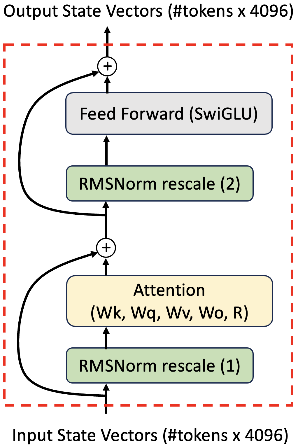
Figure 1: A Llama 2 transformer block.

The full set of matrices for Llama 2 is listed here. Let’s tally the parameters:

1. Input encoder and output layers that map between the model dimension (4096) and the token vocabulary (32000). I’ll refer to both of these 32000x4096 matrices as token ‘dictionaries’ in the text below. That’s 2 * 4096 * 32000 = 262,144,000 parameters.
2. Weight matrices for the transformer attention mechanism (Wk,Wq,Wv,Wo). These are stored as 4096x4096 tensors in the Llama 2 download, but should be thought of as 32x128x4096 (or permutations thereof), as there are 32 attention heads. That’s 4 * 4096² = 67,108,864 attention parameters per transformer.
3. It’s worth noting that these head-specific matrices act in pairs as Wv_h^TWo_h and Wq_h^TR(d)^TR(d)Wk_h, where the R(d) matrices apply relative positional encoding that depends on the distance d between key and query tokens. Each Wq_h^TR^TRWk_h pair behaves very similarly to the low rank LoRA representation of a larger 4096x4096 tensor.
4. Weight matrices for the feed forward network, which maps from the model dimension (4096) to a higher internal dimension (11008), and then back to the model dimension. This would typically involve two linear layers (4096x11008 and 11008x4096), but Llama uses a SwiGLU activation for the first layer which requires an additional matrix. That’s 3 * 4096 * 11008 = 135,266,304 feed forward parameters per transformer.
5. Note that there are 32 transformer layers, so one has 32 inequivalent versions of the matrices described in points (2-3)! Each layer also includes two 4096-long rescaling vectors within the Llama equivalent of batch normalization (RMSNorm), and I see one final rescaling operation on the last transformer output - I’ll touch on this in Section 5. There is also a vector containing 64 frequencies used to create the relative position encoding R(d) matrices. Putting it all together, we get:

  262,144,000 token dict + 64 position encoding freq + 4096 final RMSNorm +
  32 layers * (67,108,864 attention + 135,266,304 feed forward + 2 * 4096 RMSNorm) 
= 6,738,415,680 total parameters

We’ll also take a look at several internal state matrices:

1. Attention matrices (#tokens x #tokens): Each attention head creates its own attention matrix, so if a context window contains 1000 input tokens, there will be 32 heads x 1000x1000 matrices per transformer layer. However, with masked attention, only the bottom row of these attention matrices (a 1000-long vector) remains relevant for next-token generation.
2. The attention block outputs #tokens x 4096 state vectors that are added to the transformer inputs - this recombination with earlier states is called a persistent connection (see curved lines in Fig. 1). These vectors are interesting, but do not need to be cached when running the model, and are not explored closely in the current version of this document.
3. After the attention block persistent connection, the #tokens x 4096 state vectors are fed into the feedforward layer, which acts on each 4096-long state vector independently - it is not synthesizing information between the different state vectors. The feedforward layer outputs another set of #tokens x 4096 state vectors, which we’ll look at in Sections 2 and 5. Only one of these 4096-long vectors needs to be created when generating a new token, however the previous vectors all need to be cached. Counting the first layer’s input as a 33rd ‘layer’, this contributes just 270 MB to the cache for a prompt size of 1000. (270 MB ~ 33 layers x #tokens x 4096 x 2 bytes/float)

Figure 2: A Llama 2 7B attention block. State vectors (#tokens x 4096) are rescaled and slightly recentered by the RMSNorm function. Other steps follow the standard transformer architecture, with red and yellow paths linking processes that occur simultaneously for each attention head. Llama and Llama 2 use roformer (R matrix) relative positional encoding. Source code for the model can be found here, and the attention mechanism is reviewed more closely here.

2. What can we directly decode from internal states of the model?

In the subsections below, we’ll see that some of what the model is ‘thinking’ can be decoded from three separate sets of word-to-vector mappings. Information is passed forward through the model in the form of N sets of 4096-long vectors, where N is the number of input tokens. The use of masked attention in Llama-2 means that these vectors are computed sequentially. The N-1’th output of each layer is fully created before the model begins to work on the layer corresponding to the N’th token, which has access to all earlier information.

At the start and end of the model, the 32000x4096 input encoder and output layers give a direct mapping between these internal 4096-long state vectors and specific tokens (pieces of words). I’ll refer to these matrices as dictionaries, because they allow us to translate between the model state vectors and natural language words. A third dictionary (and I suspect there are more) is only found in layer outputs within the transformer stack, and seems to reveal word associations that help the model parse meaning. I’ll refer to this as the ‘middle’ dictionary.

The input and output dictionaries have significantly correlated internal structures (see Section 2A below) and meaningful interrelationships that I’ll circle back to in Figure 5. However, the dictionaries do not have word<–>vector mappings in common, so if you record a word using one dictionary, the same word cannot be read back out using another. This property means that the model can use different dictionaries simultaneously to hold multiple sets of words. The average Pearson correlation coefficient (normalized inner product of zero-mean vectors) between input and output dictionary vectors for the same token is 0.016, just as for vectors of normally distributed random numbers (0.016 ~ 1/sqrt(4096)).

The vectorization of tokens in an LLM can bake in a lot of meaning, such as the famous v_king - v_man + v_woman ≈ v_queen relation between token embedding vectors in word2vec. I haven’t been able to reproduce that sort of equation for Llama-2 7B, and there is a great reason to expect it not to hold: the final state vectors of the model represent sets of dissimilar words, and an additive logic within the closely related vector spaces – say, v_woman + v_crown = v_queen – would create problems for this. If the model wanted to consider both “woman” and “crown” as possible next-word candidates, it would end up outputting “queen” instead.

So, if that’s not how it works, what do the word encodings actually look like?

2.A. Word association in the token encoding vector spaces:

The input and output dictionaries have similar structures, by which I mean that token vectors with close meanings tend to be separated by about the same angle in both dictionaries, giving them similar inner products. Let’s take a closer look at just the input dictionary to get a sense of what these word associations look like:

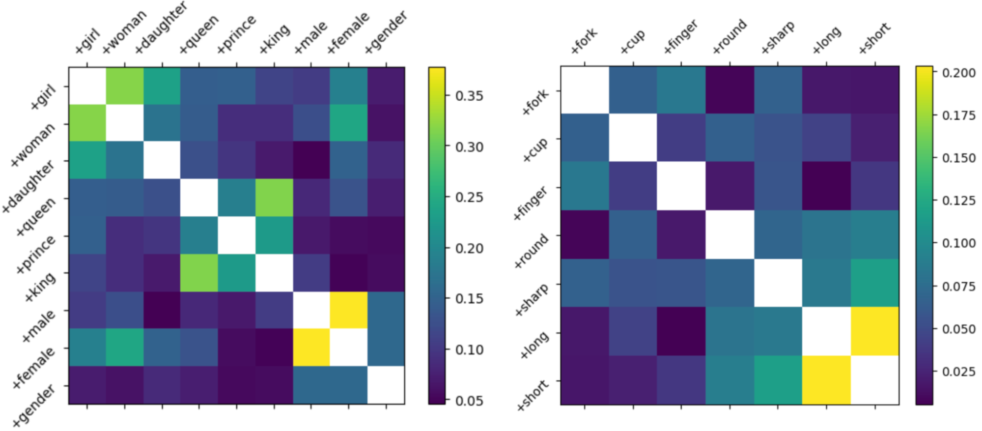
Figure 3: Similarity of input word encodings. Normalized inner products between the 4096-long encoding vectors for different single-token words. (amplitude A = <v1|v2> / sqrt(<v1|v1><v2|v2>), for vectors v1 and v2 read from the 32000x4096 input encoder layer)

The first thing that jumps out is that words with close meanings are fairly consistent in having large inner products. More than that, part of speech is a factor – the adjectives in Fig. 3 (“round”, “sharp”, “long”, and “short”) also have greater than average inner products with one another, and with other adjectives I’ve tested. Adjectives addressing a similar property (“long”/“short”, “male”/”female” “red”/”yellow”) have even closer encodings.

Some degree of correlation is unavoidable as the model’s vocabulary exceeds the state vector length, but these correlations probably serve several purposes. Shrinking the angles between vectors allows a more compact (lower effective rank) representation of the dictionary, which can reduce accidental spillover (noise) onto other information encoded in the same 4096-long state vector. Just as importantly, having a common vector component within related word-vectors could also give the key and query attention matrices (Wk and Wq) a way to identify related classes of words (say, colors) or part of speech agreement.

This structure also means that similar word-vectors reinforce one another. If you use the output dictionary to create an output vector containing an equal sum of 3 token vectors and two of them are colors, the chance of the model generating a color as the next token will be greater than 2/3! For example, defining v = v_red + v_green + v_big gives output (logit) values 1.25 = <v|v_red1> ~ <v|v_green> > <v|v_big> = 1.08, for L2 normalized single-token vectors.

It’s also noteworthy that the scale bar of Fig. 3 has only positive numbers. This wasn’t deliberate, and it turns out that token inner products are positive 81% of the time. My sense from casual examination is that they’re generally (but not universally) positive for pairings of English words or word-parts, and more often negative for English-to-foreign pairings (particularly with East Asian characters). This seems to suggest that words from different languages can behave competitively, suppressing one another’s amplitude in he output dictionary register. Here, I’m using the term ‘register’ to refer to the set of words and associated amplitudes that are found when interpreting a 4096-long state vector with a particular dictionary.

There’s an even subtler form of word association that we can’t see in Fig. 3 – words in the input dictionary tend to look like word completions in the output dictionary. For example, the input embedding of “play” has large inner products with “ground” and “offs” in the output encoding! To get into this, we’ll want to start looking at internal layers of the model.

2.B. Internal dictionaries of an LLM:

The persistent connections in the model (curved lines in Fig. 1) cause the inputs to any given transformer layer to be partially copied over into the transformer’s outputs, suggesting that the model will continue to have a relationship with the same encodings over multiple transformer layers. So… what happens when we use the input and output dictionaries to interpret state vectors (transformer outputs) from the middle of the transformer stack?

Let’s consider a short prompt containing a few clear internal word relationships: “I like the red ball, but my girlfriend likes the larger ball. We like to go to the basketball court to play ball together. It is a lot of fun.”

Using the input dictionary results in plots like these:

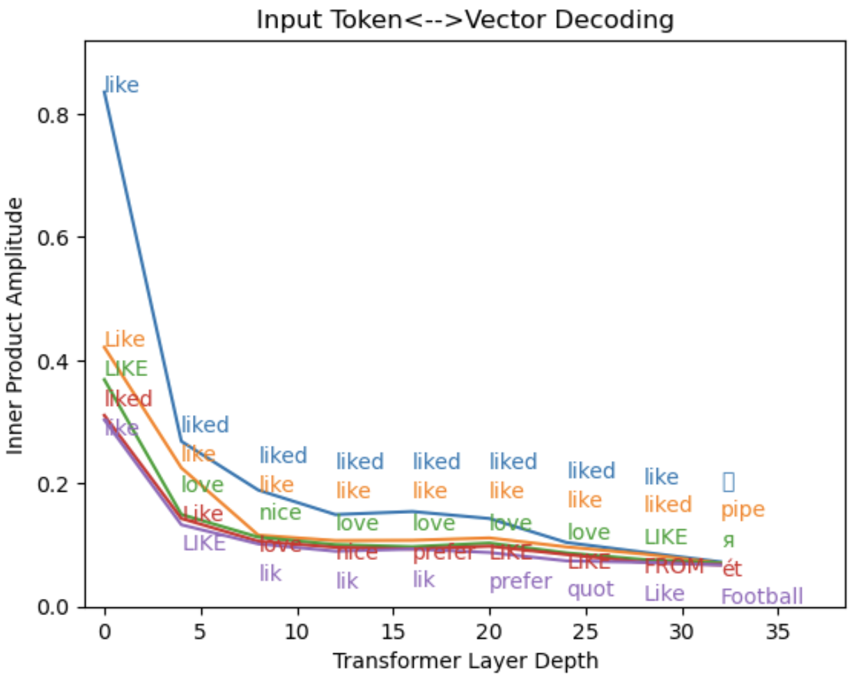
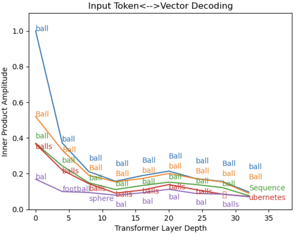
Figure 4: Reading internal states using the input encoding. Transformer output vectors (4096-long vectors) in the (top) 3rd word token=“like” position and (bottom) 6th word token=“ball” position are decoded using the 32000x4096 input encoding matrix. Amplitude of the five largest vector elements is plotted and overlaid with the words that each matrix element represents. The transformer outputs are L2 normalized, but the input encoding matrix is not.

The prompt contains 37 tokens, so the output of each transformer is a set of 37 4096-long vectors corresponding to each of the input token positions:

0: “<s>”
1: “I”
2: “like”
3: “the”

… and so on, where “<s>” is a dummy token placed at the start of every prompt. Projecting these vectors onto the input dictionary reveals that each input word continues to be readable all the way through the network. There seems to be a little drift, like conflating “ball” and “Ball”, but it’s striking that the input dictionary remains usable and the embedding of the input token is protected from exponential decay as it propagates through ~30 transformer layers. Instead of vanishing, the amplitude drops to a roughly constant level beyond the 10th layer (A ~ 0.15 to 0.2), with a weight that corresponds to A²~ 3% of the full state vector.

Things get more interested when we use the output dictionary:

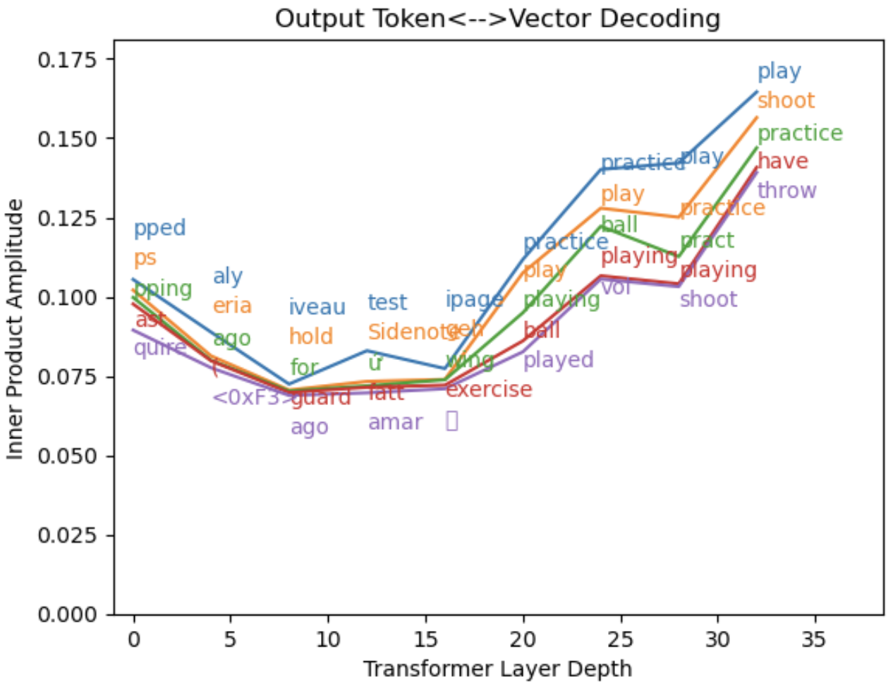
Figure 5: Reading internal states using the output dictionary. The model generates low-quality predictions with short prompts, so I’ve chosen the 25th token position to decode (“to” in “basketball court to play ball”).

Unlike the projection onto input encoding, this output projection shows us collections of words that aren’t all that closely associated, such as “shoot” and “play”. My favorite thing about this plot is the set of words in “layer 0”, which shows how the raw input encoding of “to” is read in the output encoding language. Rather than being meaningless, the “to” input vector projects strongly onto a set of tokens that can expand the word into “tops”, “topped”, “topping”, and “toast”! The input and output encodings don’t just have similar structures – they’re also nestled with one another in a way that causes the input embeddings to automatically suggest sequential tokens when read with the output encoding.

In practice, these layer 0 continuations are usually incorrect, and plots like Fig. 5 stop showing them within the first few layers. The pattern I tend to see is that plausible words start to appear around the middle of the model (layers 10-20), and the word set becomes much better informed by logic and context in the last ~10 transformer layers. A recent paper found that most factual knowledge seems to be encoded in the first half of the model, so it may be that the second half of the model is specialized in integrating context.

Here’s another example of output-based decoding that shows similar patterns:

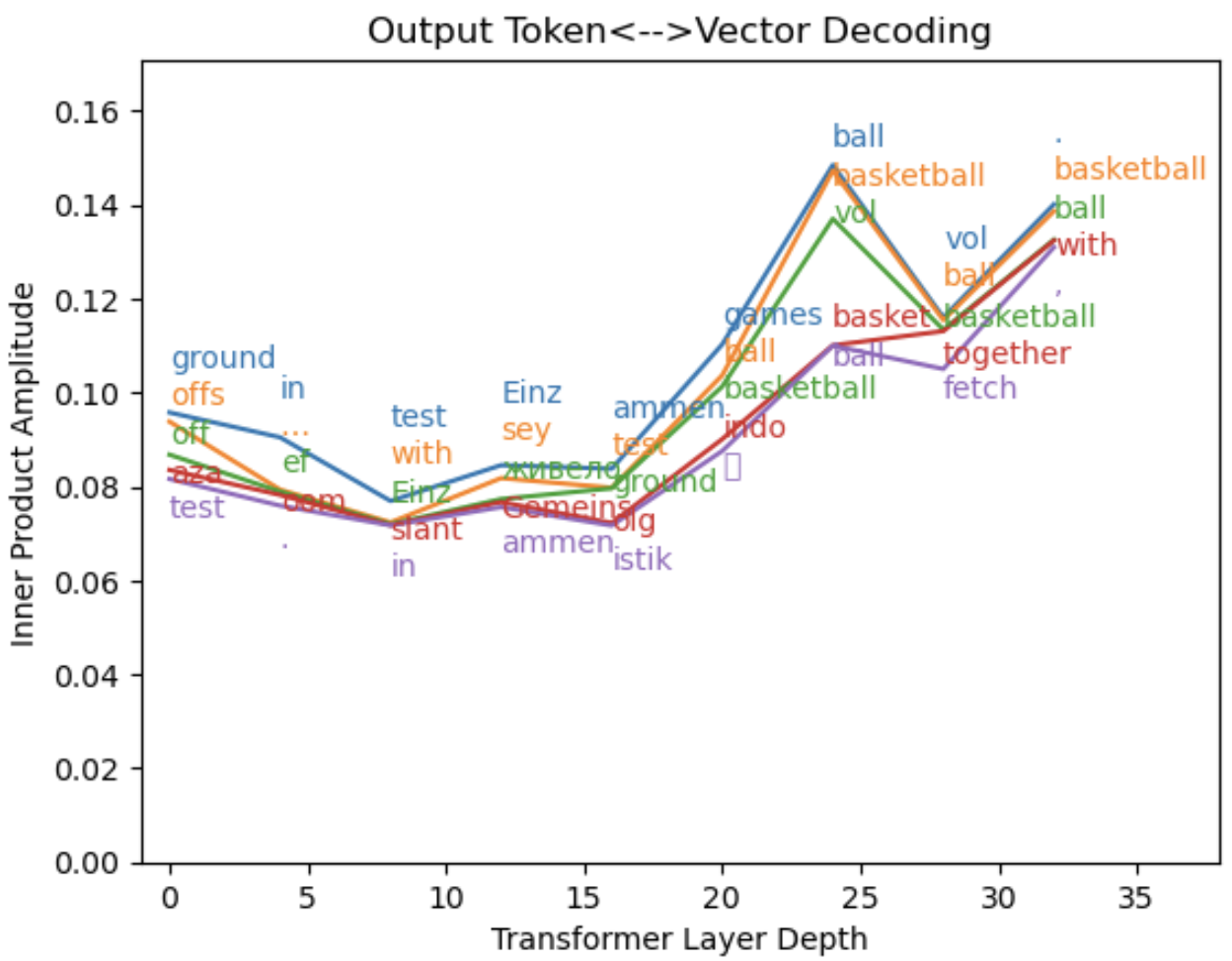
Figure 6: Reading internal states using the output dictionary. The input word is “play”, as in “basketball court to play ball”).

The decodings of the internal states in Fig. 4-6 are still missing something important. We can see that the model remembers its prompts, and we can see it spitballing ideas for the next token, but we can’t see the kind of pairwise word associations that one would expect from the key/query structure of attention. To look a little bit further, let’s create a very approximate dictionary based on how the model transforms tokens in the first couple of transformer layers (method here). I’ll refer to this as the “middle” dictionary.

Here’s what happens when we try to use it…

Figure 7: Reading internal states using the middle dictionary. The 3rd token position is decoded (“like” in “<s> I like the red ball”).

Several things stand out:

1. The middle dictionary has little overlap with the input and output dictionaries, which gives us very weak amplitudes in layers 0 (the input vectors) and 32 (the final state vectors). This is not an entirely trivial observation – it suggests that the model has opened up an isolated sector of its 4096-dimensional state space. By “isolated”, I mean that it seems like vectors in the middle dictionary do not closely resemble specific vectors in the other dictionaries.
2. Unlike the input and output dictionaries, the middle dictionary shows us the previous word in the sentence - “I”! Due to the attention masking within Llama and GPT-family models, the layer outputs in the 3rd token position (“<s> I like”) are only aware of the input tokens “I”, “like”, and the dummy token “<s>”. I’ve removed <s> from the middle dictionary basis by hand, and the remaining words “I” and “like” are both visible in this middle encoding register.
3. Words that are modestly related to “I” show up with similar amplitudes, including “We”, “my”, and fellow pronoun, “it”. This is probably partly because of inaccuracy in the method used to identify the “I” vector, but it’s also possible that meanings in the middle dictionary do not exactly map to single-word meanings within natural language.

To mitigate the inaccuracy of the middle dictionary, we can limit the basis to just the 28 unique tokens that exist in the prompt. Here’s what that looks like for the 6th token position:

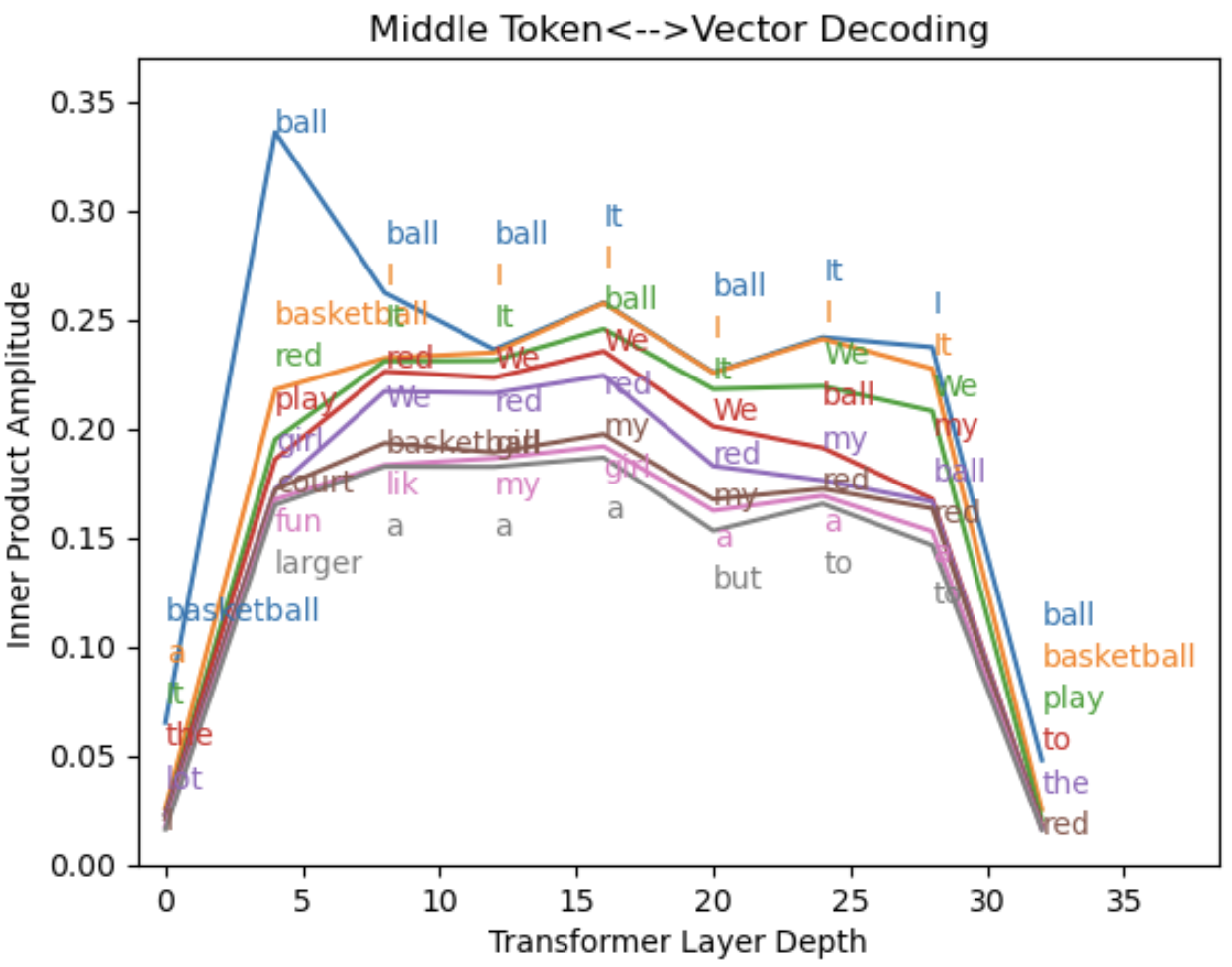
Figure 8: Reading internal states using the middle encoding. The decoded token position corresponds with “ball” (“<s> I like the red ball”). The top eight word matches are plotted.

The words “I”, “red” and “ball” are near the top of the list, possibly labeling the ball as a “red ball”. However, the confusion between “I”, “We”, “my” and “it” fills up most of the top of the displayed word list, making the plot difficult to read.

This dictionary would be easy to improve, but a central problem is that we don’t know what the model is using it for or how similar it really is to the input and output dictionaries. I would assume that the middle dictionary vectors include relational information between different words, or other nuances that we’re missing in this brute force translation. There are more computationally intensive approaches that could be used to try to dig this out, but let’s move on for now.

3. What words do the attention heads look for?

The four weight matrices (Wk, Wq, Wv, Wo) are each stored as 4096x4096 tensors in the Llama-2 download, but are partitioned into 32 128x4096 “attention head” tensors (Wk_h, Wq_h, …) when the model is run. A heatmap representation of one of these matrices can be viewed here, together with a few notes on the features visible by eye.

One starting point to dissect these matrices is to think of each attention head as containing 128 4096-long vectors that store words. The attention heads function by taking inner products between these vectors and the token encodings, so decomposing them on the input dictionary basis will give us a sense of the words that the first transformer layer is drawing connections between. In doing this, we should remember that due to the structure of the attention matrix (the attention mask), the ‘key’ vectors will be associated with tokens that occur to the left of the ‘query’ vectors.

The very first head is a great example. For head [0] (code output here), the key vectors map strongly to open parentheses and words that frequently open a parenthetical note such as “although”, “occasionally”, “approximately”, “File”. This head also looks for word endings such as “ingly”, “demic”, and “aneous” that have similar associations – think “(amazingly, …”, “(surprisingly, …”, “(simultaneously, …” and so on. The corresponding 0-indexed head query features closing parentheses, in keeping with the ‘key tokens to the left, query tokens to the right’ principle. Head [5] does something similar for quotations.

Attention heads appear play a role in linking together words that are written using multiple tokens. An aparent example is shown here for head 2 of layer 0. In principle, one could either track the output of specific attention heads or use an approach similar to the middle dictionary creation algorithm to get a sense of the embedding vectors assigned to composite words.

However, it’s overly simplistic to think of the head vectors as only searching for single words. As things stand, it’s unusual to see a single word with more than a ~30% projection onto a given 4096-long vector within Wk or Wq, so if we do think of these vectors in terms of a ‘word’ basis, we need to at least think of each one as the sum of multiple word-vectors, rather than just a single word.

We’re also glossing over the positional encoding, which modifies the key-query inner product in a way that allows the model to look for specific kinds of positional correlations. The full matrix element (added to the attention matrix at the matmul stage in Fig. 2) is <v_1|Wq_h,i^TR(d)^TR(d)Wk_h,i|v_2>, where i runs from 0 to 127 and selects pairs of 4096-long vectors for the key and query. The positional encoding R(d)^TR(d) renders different parts of the 4096-dimensional vector space senstive to different components of a Fourier transform in terms of the distance d within the prompt between a key token ‘1’ and query token ‘2’. Some attention heads seem to be primarily position sensitive, such as head 15 of layer 5 (noted in Fig. 10), which appears to always place most of its attention weight on the token that immediately precedes a query (d=1).

An alternative starting point based on the correlations in Fig. 3 may be to consider that the angles separating vectors with similar meanings or parts of speech tend to be significantly smaller than 90 degrees (typically ~65^o - 80^o, going by examples in Section 2A). Some key/query vectors may pointing towards the centers of these loose ‘clusters’ – for example, to look for related adjective/noun pairs.

It should also be noted that even though Llama-2 is a language model, the information encoded in model parameters is not purely linguistic. For example, a fascinating recent paper showed that some neuron activations (state vector components) inside the Llama models can encode values along continuous dimensions such as time and latitude/longitude.

4. How do the parameters of deep and shallow layers differ?

Let’s step back from decoding meaning and take a look at the parameter values. The distribution of Wk/Wq/Wv/Wo values is approximately 0-centered, and evolves from a fat-tailed distribution in the first (‘shallowest’) transformer layers towards a gaussian distribution as one goes deeper into the network. A great metric to track this trend with is the ratio of standard deviation to the mean amplitude [σ/mean(abs(vect))], which has a value of ~1.25 for a 0-centered gaussian.

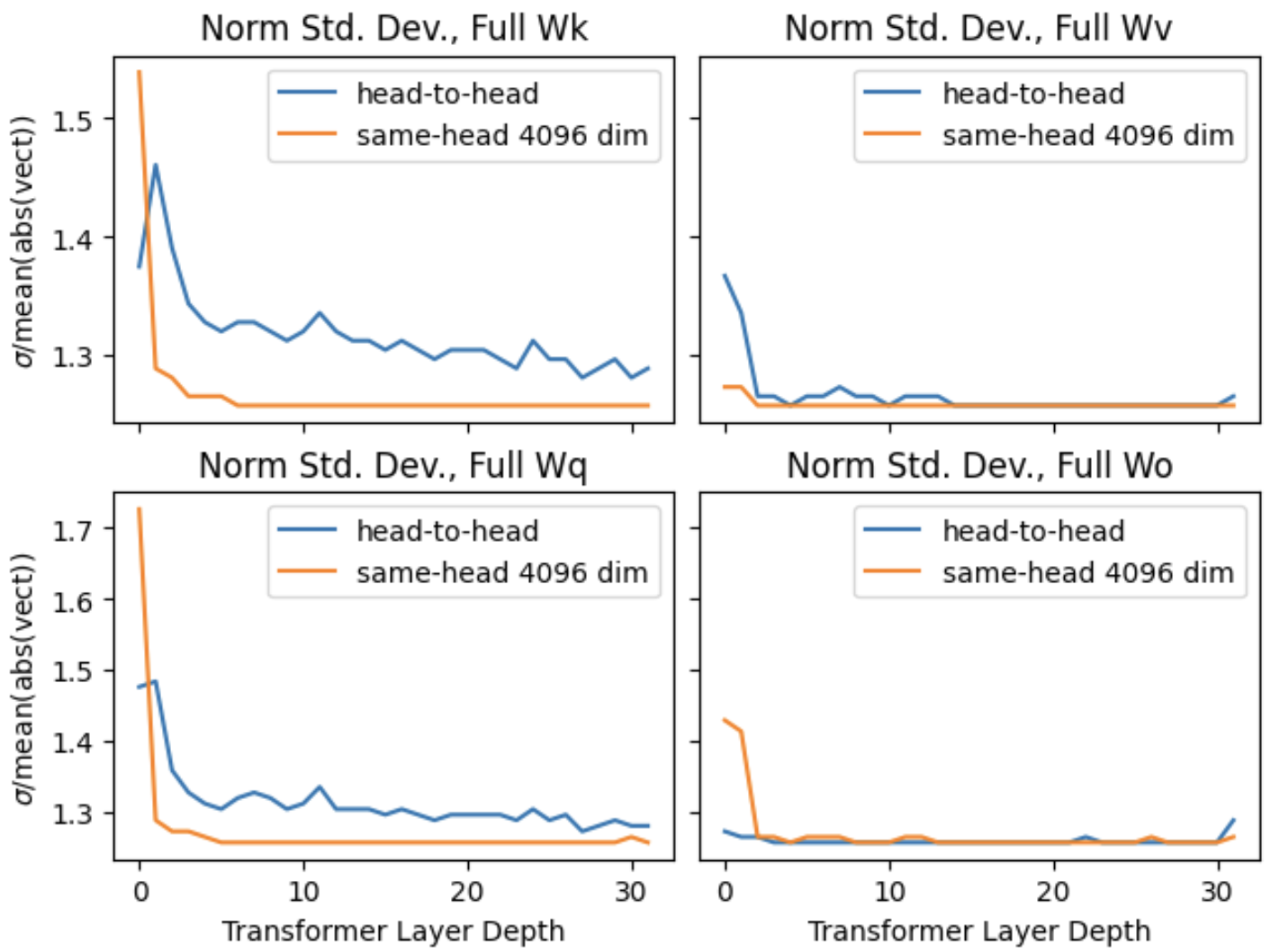
Figure 9: Parameter distribution by layer. Tracking the metric σ/mean(abs(vect)) versus layer in the neural network for 4096x4096 representations of the Wk, Wq, Wv, and Wo attention matrices. Orange curves show the mean value for vectors oriented along the 4096-long model dimension, while blue curves show the mean value for 4096-long vectors that cut across the attention heads.

Parameters in the relatively ‘overloaded’ Wk and Wq matrices have larger deviations from a gaussian distribution. I call these matrices ‘overloaded’ for two reasons: (1) because they are multiplied together before a nonlinear function (softmax) in a way that resembles the low rank LoRA representation of a larger dense neural network layer (exactly identical to LoRA for identical key and query token indices); and (2) because they need to directly parse the embeddings of both position and token vectorization.

The highly non-gaussian distribution seen in the first two layers may suggest that they are subject to more constraints than later layers. The first two layers significantly transform the state vectors (see Fig. 12 in the next Section), unlike most later layers that appear to enact smaller incremental changes. One can also note that the first layer needs to interface directly in a lossless way with input that is highly structured and specific on a per-token basis, unlike later layers in which information is distributed across the token-axis of the state vectors (transformer outputs).

5. What do the internal states look like?

This section will take a closer look at the attention matrices (32 layers x #tokens x #tokens) and the layer output state vectors (33 layers x #tokens x 4096). Note that even though there are only 32 transformer layers in the Llama 2 7B model, there are 33 sets of state vectors, as the first set of state vectors (“layer 0”) come from the initial token–>vector encoding. This section will explore structural properties that define how the model functions as an analog computer, in contrast to Section 2B, which looked at information that can be directly decoded from the state vectors.

5.A. The attention sink: stabilizing the context window

There’s an infinite amount to say about internal states, but I want to kick things off by looking at the attention sink phenomenon identified in this paper [Xiao et al., Sept. 2023]. They observed that attention connecting back to the first token tends to be extremely strong (>~0.5 out of a max of 1) beyond the first two transformer layers. Here’s the figure from their paper:

---

---

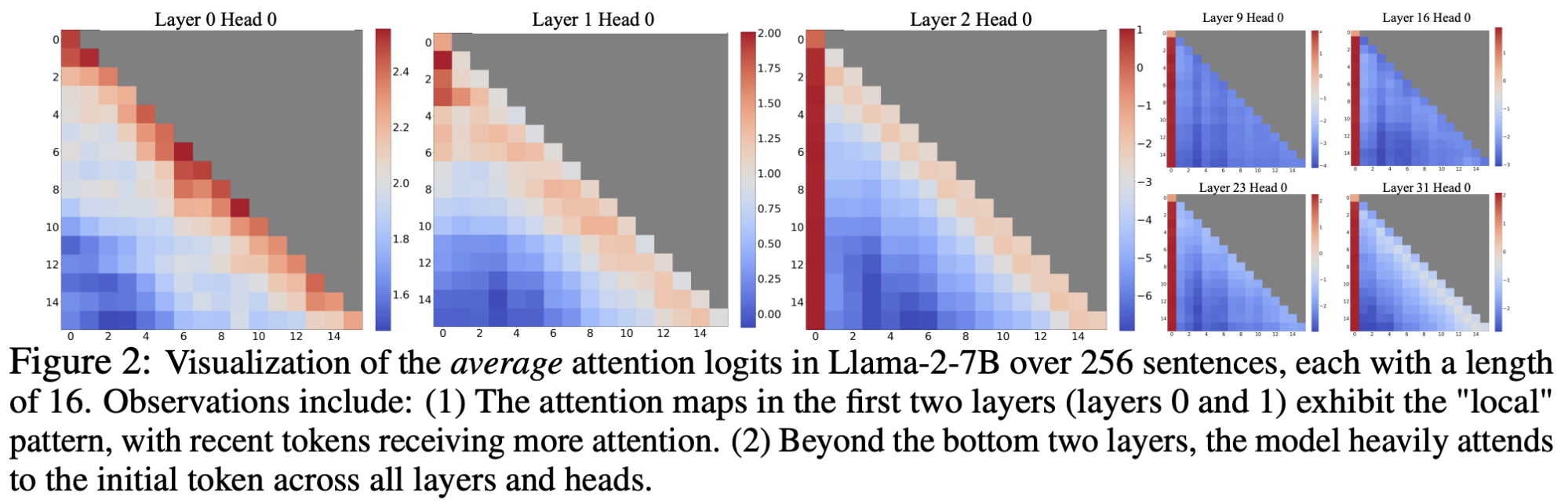
This isn’t because of specific information in the first token. The first token (<s>) is just a padding token, and the first 1x4096 token output of each layer is the same regardless of the prompt. Instead, the authors propose: “We attribute the reason to the Softmax operation, which requires attention scores to sum up to one for all contextual tokens. Thus, even when the current query does not have a strong match in many previous tokens, the model still needs to allocate these unneeded attention values somewhere so it sums up to one.”

The figures below show a couple of examples of how this plays out for a specific prompt (see captions):

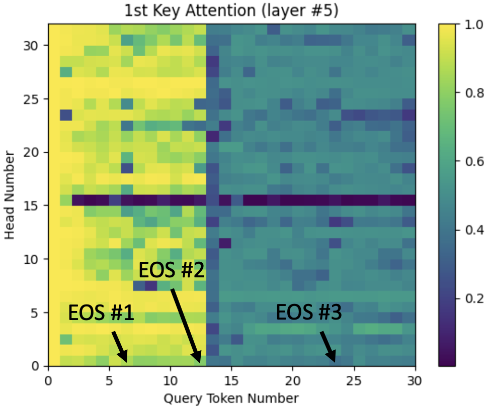
Figure 10: Attention sink effect versus output token. Attention to the first token is shown for each attention head in transformer layer #5. The end of each sentence (‘?’ character) is identified with arrows. The prompt was: “Hey, are you conscious? Can you talk to me?\nI’m not conscious, I think?\nWhat should we talk about?”

We can see the attention sink effect as advertised, but a couple of things jump out:

1. Attention head #15 in layer #5 is represented by a black row. This means that it’s not sinking attention (much) onto the first token. Instead, the attention from this head goes almost entirely to the token that immediately precedes each query (not shown).
2. The attention sink effect becomes much weaker immediately after the 2nd question mark. In fact, the effect declines significantly at the end of the first sentence (or 2nd if they’re short) in all of the the tests I’ve done, usually coinciding with a sentence break. Here’s another example. This suggests that the 1st sentence is viewed differently from others by the model, and may relate to a common role of the first sentence in providing context for everything that follows. Attention to the 1st ‘dummy’ token will cause a known vector to be copied over to later token outputs, and may even be something the model uses to highlight meaningful tokens.

One sees the very similar effects in deeper layers such as layer #25:

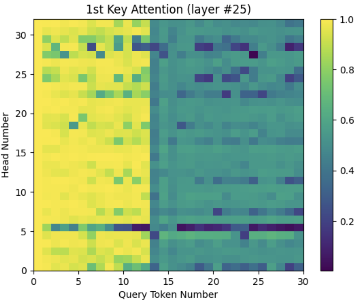
Figure 11: Attention sink effect versus output token in layer #25. Other details are as in Fig. 10.

The first sentence is consistently highlighted as seen in Fig. 10-11, but I haven’t spotted any other highlighted sentences in long prompts. Instructing the AI to assume a new role (to go from an assistant to a lawyer or famous person, etc), doesn’t seem to do it, and nor does telling it that the next sentence will give it a new role. Artificially adding a second instance of the first “dummy” token later in the prompt creates a second attention sink that sharply decreases the attention between all later query/key combinations, but it fails to result in a second highlighted sentence.

NOTE ADDED 10/26/2023: this later post adds context to how the 1st sentence is highlighted and what it may mean. It turns out that the model has converted the first sentence-ending punctuation into a second kind of attention sink token. The existence of these attention sinks highlights an interesting property of large language models: they have limited tools to manage their state vectors or introduce known vector components. The two attention sink tokens serve this purpose, and my suspicion is that they may be part of a broader internal markup language that helps the model parse text.

5.B. The state vectors: RAM of an analog computer

So, what can we say about the state vectors themselves? The simplest thing to ask is, how similar are the state vectors output by a given layer to the output of the next layer? Enter Fig. 12:

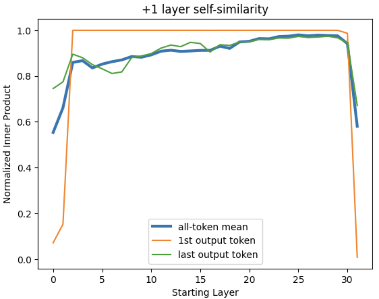
Figure 12: Self-similarity between the output of adjacent transformer layers. Normalized inner products between the 4096-long state vectors in each layer and the same-token state vectors of the next layer.

Surprisingly, transformer output is mostly identical from one layer to the next. If we exclude the first two layers and the last layer, the average normalized inner product between each layer’s input and output is 0.92. The first two layers buck this trend, but they’re highly variable depending on the token (standard deviation σ = 0.25 and 0.16). The last layer sees a large drop in correlation to 58% in this example, suggesting some significant final massaging of the vectors. Still, a naive take corroborated by Fig. 5-6 would be that the vectors defining word output are mostly settled by several layers before the end of the network.

Other than the last two layers (which I’ll get back to), the trend in Fig. 12 is about what one expects to see as information that was memorized during model training is loaded into the state vectors. I’ll take a moment to play this out, as it’s a nice window into how the state vectors act as a kind of random access memory for the model. Each state vector begins as the representation of a single token, and we can imagine a simplified scenario in which each layer of the network adds a few new token representations to the state vector (say, 3), while preserving the overall amplitude of each token-vector. This means that the initial state of a token vector would be v_0 = v_token0, and the first layer output would include two more tokens (v_1 = v_token0 + v_token1 + v_token2 + v_token3), the second layer output would encode ~5 tokens (v_2 = v_token0 + v_token1 + v_token2 + v_token3 + v_token4 + v_token5 + v_token6), and so on. Normalizing the state vectors for appropriate comparison gives a next-layer inner product of <v_i|v_i+1> = sqrt((3i+1)/(3i+4)) between layers ‘i’ and ‘i+1’. This rapidly converges towards 1, with initial values of <v_0|v_1> = 0.5, <v_1|v_2> = 0.76, and <v_2|v_3> = 0.84 that closely resemble the average trend in Fig. 12 (blue curve).

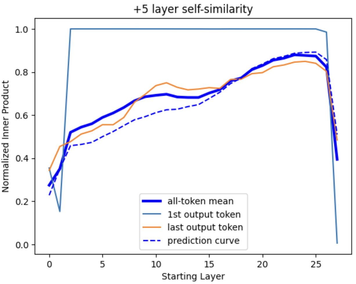
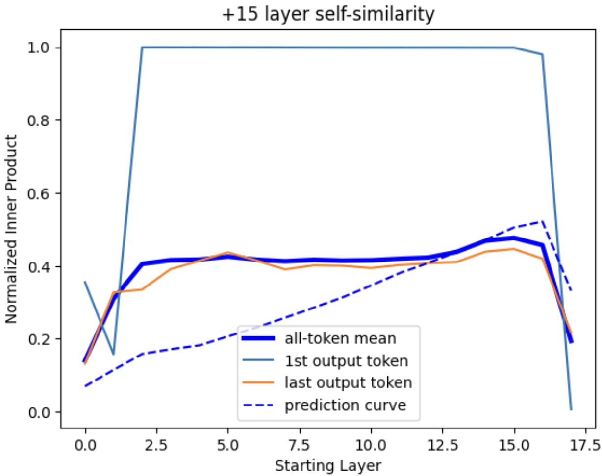
Figure 13: Self-similarity of token outputs over longer distances. Equivalent plots to Fig. 12, but with (top) 5- and (bottom) 15-layer gap between the compared vectors. A dashed prediction curve has been added showing the expected trajectory of the mean curve if single-layer inner products were multiplied together over the indicated distance.

If we skip forward a few transformer layers, we find that state vector correlations initially resemble a prediction curve (dashed line in Fig. 13, top) that represents the exponential decay-like trend expected if each layer contributed random changes. However, over longer distances, the level of correlation is significantly higher than this would predict, consistent with our observation in Section 2B that the model actively preserves certain kinds of information such as the input token. The “attention sink” coupling to the first ‘dummy’ token is also identical from layer to layer, but is not a large factor in Fig. 13 as the correlation between the dummy token state vector and other token-resolved state vectors tends to be just ~10%, and largely vanishes in the inter-layer inner product.

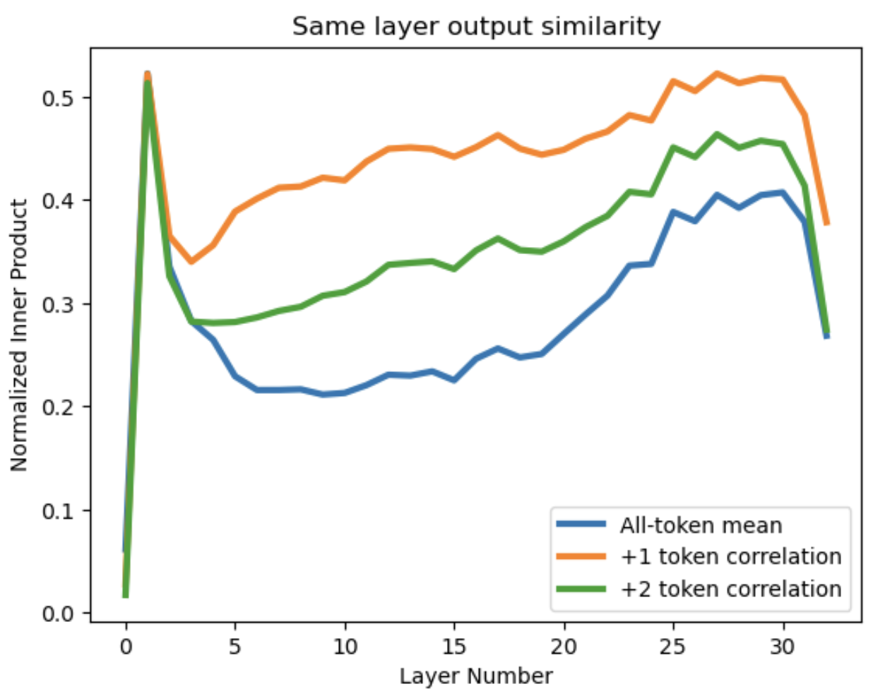
Figure 14: Similarity of state vectors in the same layer. Normalized inner products between (orange) neighboring-token state vectors and (green) next-neighbor vectors are compared with (blue) the average over all non-identical token vector pairs (mean distance of 10.3). “Layer #0” represents the encoded input tokens prior to the first transformer layer.

Different token state vectors of the same layer also look somewhat similar to one another all the way through the network (Fig. 14), and similarity is notably higher when token indices differ by <~3. Other short prompts (up to ~200 tokens) that I’ve tried yielded essentially identical trends, and even showed some of the same noise-like jitter seen in Fig. 14.

This is getting long, but one last figure!

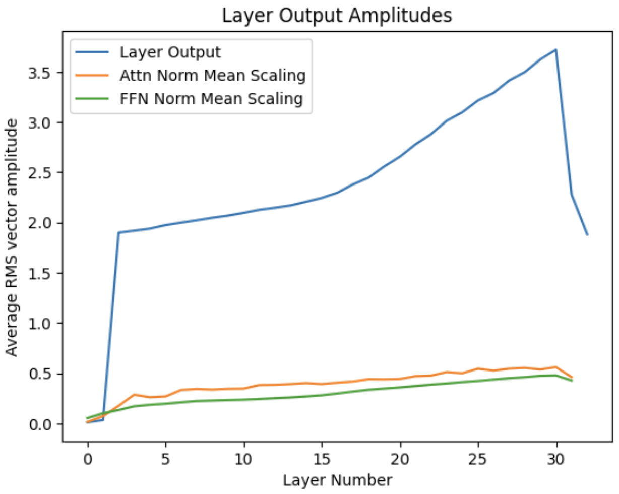
Figure 15: Layer output RMS amplitude and the mean value of RMSNorm scaling parameters.

As a final nuance, I want to note that the amplitude of the state vectors isn’t constant across the network (Fig. 15). They tend to grow larger, and there are strikingly large slopes in the first two and last two layers. A first guess would be that this progressively growing amplitude will weaken (or break at layer 2-3) the residual connections, but the scaling of transformer input (RMSNorm layer inputs) also grows with depth in the layer, and should counteract some of this effect. Also, the RMSNorm vector that rescales amplitudes going into the attention block of the first transformer layer are tiny and can even be negative – their interplay with the first two layers warrants a closer look.

6. Lessons for LLM architecture

A few impressions:

1. The model is performing analog computation, so it is important to understand the effective “noise” that disrupts the fidelity of encoded information. There are clear noise issues with the fidelity of information read by the input, output, and middle dictionaries, but one can’t tell if this is noise in the model or just an issue with the dictionary.

   A simple interpretation of this would be that because the model is using multiple dictionaries, any incomplete orthogonalization between the dictionary vector spaces will cause words used by one dictionary to come across as noise for all the others. This gives the model strong motivation to compress the effective rank of each dictionary matrix (such as the 32000x4096 input encoding), though the overlap between the dictionaries also has a meaningful structure as we saw in Fig. 5-6.

   In practice the dictionaries are not very compressed in rank (see SVD figure), and not really possible to orthogonalize. The tradeoff the model seems to have accepted is that each dictionary register specifies words very precisely, but contains just a few intelligible words and has a high noise floor. My sense (from expanded versions of Fig. 4-6) is that the words devolve into senselessness beneath a critical amplitude of F ~ 0.07. Some of the perceived noise could be due to drift in the underlying meaning-to-vector mappings of a given dictionary, as they don’t need remain constant across the tranformer stack. But F ~ 0.07 is roughly consistent with the value of ~0.06 that one would expect if you approximate words from other dictionaries as having random normally distributed 0-mean vector elements. I’m associating the noise floor with the minimum amplitude value beyond which the number of words that one expects to observe from noise alone [4096 * (1 - erf(F / (σ * sqrt(2)))) / 2] rounds to 0, which amounts to satifying the inequality: 4096 * (1 - erf(F * sqrt(4096 / 2))) < 1

2. A bold interpretation of point (1) would be that model dimension (4096 for Llama 2 7B) defines the scope of the model’s ‘inner monologue’. If we extrapolate from a noise floor of F=0.07, each 4096-long token vector within the model could contain an absolute maximum of N~200 legible embedded words (200 ~ 1/0.07², as normalization gives N * A² ~ 1). However, even the amplitude of ‘illegible’ words could be relevant to performance of the model, and as successive transformers adding weakly to the amplitude of an illegible word can eventually bring it through the noise floor. It’s worth remembering that output amplitudes shift quite slowly from one transformer layer to the next, and the middle of the model (16th layer output) already has a ~0.2 average correlation coefficient with the final output.

   Another way in which words beneath the noise floor can remain relevant is if the model is primarily using just one dictionary. This appears to be the case for the model’s final output, which projects only weakly onto the input and middle dictionaries. In this scenario, the word associations built into the dictionary are likely to cause tokens (logits) identified beneath the nominal noise floor to preserve significant similarities in meaning and part of speech with the higher value tokens. (higher value logits)

3. Attention to the first token – the attention sink phenomenon – seems to act as a highlighter for the first sentence, rather than just a ‘sink’. I’m assuming that the first sentence would be highlighted rather than ignored, as it’s the first context the model gets, but it’s also possible that the model has just adapted to ignore redundant initial prompts.

   It would be interesting to try manually manipulating attention to the first token (or weight from the 1st token Wv vector) in the context of prompt engineering, as a way to highlight important instructions. Looking quickly (plot here), I see that there’s some positive correlation between the attention sink amplitude and output amplitude in the first ~10 layers of the transformer, which could be consistent with a highlighting effect, but later layers have a negative amplitude.

4. The first sentence highlighting function touches on a fascinating question: how does the model manage so well for vastly different numbers of prompt tokens (say, 20 versus 2000)? The model is applying the same kind of processing to inputs regardless of the prompt length, but maintaining coherence is a finely tuned balancing act. Perplexity skyrockets if you try to extend the prompt length beyond the trained context window. Amplitude of coupling to the attention sink gradually decays for longer prompts, and it’s easy to speculate at roles that this may be playing to help stabilize model behavior.

5. The strong similarity between state vectors with different token indices (30+% correlation for later layers [checked with a longer ~200 token prompt]) makes me wonder how the model harmonizes its state when information from later tokens sharply contradicts or recontextualizes interpretations based on the earlier tokens. This sort of scenario seems likely to generate bottlenecks for the masked attention architecture of current generative LLM, in which each token output is unaware of later tokens in the stream.

6. This is a very rough generalization, but the first half of the model seems to be specialized in grammatical parsing and memory retrieval, while we mostly see thoughtful and context-informed updates to the output coming through in the last 1/3rd or so of the transformer layers. The last two layers purge content stored using the non-output dictionaries, which can be expected to remove a great deal of nonsensical ‘noise’ from the model output.

7. The gaussian parameter distributions in the encoder and deeper attention layers is a striking feature, and gaussian distributions are also seen in the feedforward network. My very shallow take is that there’s a vast set of similarly optimized states, and the convergence towards one of these probably looks like a random walk with respect to the basis we’re observing from.

   A corollary to this would be that when the distribution is highly non-gaussian, the solution set is probably more constrained. This would make me leary of using a low rank fine tuning technique like LoRA. We see non-gaussian distributions in weight matrices for the 1st two layers, and to some extent in the Wk and Wq matrices throughout the network.

7. Useful links

Here are some helpful references:

1. Matrix definitions for the attention mechanism.
2. Pytorch code defining the Llama 2 neural network can be found here.
3. The Llama 2 release paper.
4. The excellent “Let’s build GPT” tutorial by Andrej Karpathy (2 hours).
5. I’d recommend starting here if you want to run a quantized Llama-2 model on your own computer. Here’s a link to my bare-bones GUI, which includes AI editor agents for a collaborative text generation experience.
6. Jupyter notebooks used to generate most of the output are available upon request.

---

<

Blog Archive

Archive of all previous blog posts

>

Next Post

Llama surprises